Scroll 8: Djoser's Discoveries
Welcome to Scroll 8, the grand finale of the Djoser’s Bulk RNAseq Tutorial Codex.
In this closing chapter, we rise above lists of genes and zoom out to see the entire landscape of biological activity. Here, we harness the power of Gene Set Enrichment Analysis (GSEA), a method that evaluates whether predefined groups of genes, such as those linked to specific pathways or biological functions, are consistently up or down regulated in our dataset.
GSEA allows us to detect subtle but coordinated changes that might be missed when looking only at individual genes. This approach offers an Eagle Eye View, revealing how groups of genes act together to influence the biology of our conditions.
Like Djoser, whose innovative step pyramid forever changed the architectural skyline of ancient Egypt, GSEA enables us to build upon our previous findings and see the structured, layered patterns that underpin our data.
It’s time to climb to the very top and take in the full view.
📜 Scroll Objectives
- Gene Set Enrichment Analysis
- Why We Use GSEA?
- Performing GSEA
- Interpreting GSEA Results
- Cultural Spotlight: Djoser & Egypt’s First Pyramid
- Codex Conclusion
Gene Set Enrichment Analysis
Gene Set Enrichment Analysis (GSEA) is a computational method used to determine whether predefined sets of genes (often representing biological processes, pathways, or functional categories) show statistically significant differences between two biological states or conditions, for example, treated vs. untreated or disease vs. healthy samples.
Instead of focusing only on individual differentially expressed genes (DEGs), GSEA evaluates entire gene sets. This allows it to detect subtle but coordinated changes in groups of related genes, even if individual genes do not pass conventional thresholds for significance.
Why We Use GSEA?
- Captures coordinated changes: Biology often acts through groups of genes rather than isolated ones. GSEA detects patterns that single gene analysis might miss.
- Reduces bias from arbitrary cutoffs: Many genes with moderate but consistent expression changes can be biologically meaningful. GSEA includes them by looking at ranked gene lists instead of hard DEG thresholds.
- Provides biological context: By linking gene expression changes to known pathways, molecular functions, or biological processes, GSEA helps researchers interpret the data in terms of real biological mechanisms.
- Enhances reproducibility: Pathway level signals tend to be more consistent across experiments than individual genes, making GSEA findings more robust.
Performing GSEA
Prerequisites: You should have a DESeq2 results table (e.g., res.df) that includes gene identifiers (e.g., gene_name) and an effect size/statistic (e.g., log2FoldChange).
Important: For GSEA you should rank all tested genes, not just DEGs. Use the unfiltered results (before applying padj/log2FC cutoffs).
🔹 Step 1: Prepare a ranked gene list
GSEA works by evaluating whether members of a predefined gene set tend to occur toward the top or bottom of a ranked list, rather than being randomly distributed. This ranking is essential because it defines the order in which GSEA “walks” through the genes, calculating an enrichment score based on the cumulative presence of the set members.
Gene Ranking Options
Most common ones include:
- log2FoldChange (magnitude & direction) (Used in this tutorial)
- signed statistic (e.g., stat from DESeq2, or sign(log2FC) * -log10(pvalue))
Some workflows rank by a signed statistic (e.g., stat from DESeq2, or sign(log2FC) * -log10(pvalue)) because it blends effect size + significance.
1
2
3
4
# Step 1: Prepare ranked gene list
ranks <- res.df$log2FoldChange
names(ranks) <- res.df$gene_name
ranks <- ranks[!is.na(ranks)] %>% sort(decreasing = TRUE)
res.df$log2FoldChange: we use the log2 fold-change as the ranking statistic (magnitude & direction).names(ranks)<- res.df$gene_name: assigns gene symbols as names;fgseaexpects a named numeric vector.- Remove NAs and sort decreasing: required by
fgsea(largest positive changes first).
🔹 Step 2: Fetch MSigDB C2 KEGG gene sets
1
2
3
4
5
6
7
8
9
10
11
library(msigdbr)

# Step 2: Fetch MSigDB C2 KEGG gene sets
hs_gsea_c2 <- msigdbr(
  species      = "Homo sapiens",
  collection   = "C2",
  subcollection = "KEGG_LEGACY"
) %>%
  dplyr::select(gs_name, gene_symbol)

pathways <- split(hs_gsea_c2$gene_symbol, hs_gsea_c2$gs_name)
msigdbr(...): pulls curated gene sets fromMSigDBfor human.collection = "C2": curated gene sets (literature/pathway based).subcollection = "KEGG_LEGACY": KEGG-based sets mirrored inMSigDB(the “legacy” subset).
We keep only
gs_name(set name) andgene_symbol(members).
split(...): converts the long table into a named list of pathways, where each element is the vector of gene symbols in that set. This is exactly the formatfgsea()needs.
There are other alternative gene sets that can be used as well like
Hallmark setsandREACTOME.
🔹 Step 3: Setting a Seed
GSEA involves permutations (either of phenotypes or gene labels) to calculate enrichment significance. These permutations are inherently random, meaning that if you run GSEA multiple times without fixing a seed, the exact p-values and enrichment scores can vary slightly. Setting a seed (e.g., set.seed(123) in R) locks the random number generator to a fixed state, ensuring reproducible results.
This is crucial for:
- Scientific reproducibility (so others can get the same results from your code).
- Debugging and comparisons between different ranking or filtering strategies.
- Avoiding confusion if results shift slightly between runs.
1
2
# Step 3: Setting a Seed
set.seed(123)
🔹 Step 4: Run GSEA with fgsea
1
2
3
4
5
6
7
8
9
10
library(fgsea)

# Step 4: Run GSEA with fgsea
fgsea.res <- fgsea(
  pathways = pathways,  # gene symbols of our fetched MSigDB C2 KEGG gene sets
  stats    = ranks,     # our ranked genes
  minSize  = 15,        # ignore tiny gene sets (reduces false positives)
  maxSize  = 500,       # ignore very large sets (too generic)
  nperm    = 10000      # number of permutations; higher = more stable p-values
)
pathways-> is the list of pathways we fetched fromMSigDBstats-> ourlog2FoldChangeRanked Gene setminSize-> Excludes pathways containing fewer than 15 genes from analysis (Reduces False Positives).maxSize-> Excludes very large pathways (more than 500 genes) which can make results less biologically specific.nperm-> Number of permutations to compute the p-value (Higher values = more stable).
As Always we will convert the results into a tidy format for easier interpretation and visualization and filter the significant ones (padj < 0.05 & abs(NES) > 1).
1
2
3
4
# Process results
fgsea.df <- as_tibble(fgsea.res) %>%
  arrange(padj) %>%
  filter(padj < 0.05, abs(NES) > 1)
NES (Normalized Enrichment Score): it measures enrichment strength relative to gene set size and distribution.
To make it very simple: Since we ranked our genes in descending order, this places upregulated genes at the top and downregulated at the bottom, so positive NES pathways are upregulated and negative NES pathways are downregulated.
Interpreting GSEA Results
Interpreting GSEA output is conceptually similar to how we interpreted GO and KEGG enrichment results in the previous scroll Thutmose’s Trends (Functional Enrichment Analysis), but with a twist: instead of focusing only on a subset of significantly differentially expressed genes, GSEA considers the entire ranked list.
Key points for interpretation:
- NES (Normalized Enrichment Score):
Indicates the degree to which a gene set is overrepresented at the top (upregulated) or bottom (downregulated) of the ranked list, normalized for gene set size. - FDR q-value:
Adjusted p-value that accounts for multiple testing; lower values mean higher confidence in the enrichment. - Positive vs. negative NES:
- Positive NES → genes in the set are mostly upregulated.
- Negative NES → genes are mostly downregulated.
Connection to GO & KEGG results:
- Like GO/KEGG, GSEA identifies biological themes/pathways enriched in your dataset.
- The main difference is no arbitrary cutoff, it captures subtle, coordinated shifts that GO/KEGG might miss if the fold change isn’t large enough.
Visualization of GSEA Results
We can use plotEnrichment() to visualize the enrichment results for specific gene sets.
Here is an example code of producing an Enrichment plot of the top pathway of our GSEA results:
1
2
3
4
5
6
7
top_pathway <- fgsea.df$pathway[1]
plotEnrichment(pathway = pathways[[top_pathway]],
               stats = ranks) +
  labs(title = top_pathway,
       subtitle = paste("NES =", round(fgsea.df$NES[2], 2),
                        "p.adjust =", format(fgsea.df$padj[2], scientific = TRUE, digits = 3))) +
  theme_minimal()
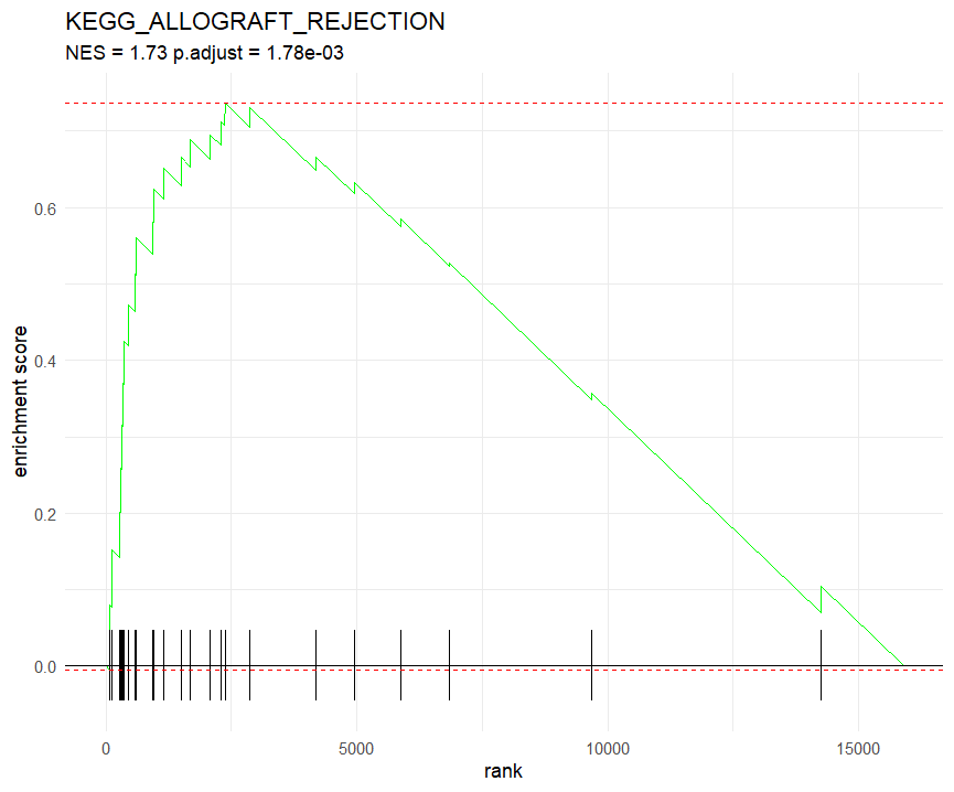
GSEA Enrichment Plot - KEGG_ALLOGRAFT_REJECTION
- on the X-axis, we have the gene rank, indicating the position of each gene in the ranked list.
- on the Y-axis, we have the running enrichment score (ES), which reflects the degree of enrichment of the gene set as we move through the ranked list.
- Our top Enriched pathway is
KEGG_ALLOGRAFT_REJECTION. - we can clearly see the enrichment score peaking (green lines) at the beginning of our ranked list as well as bottom black ticks indicating the positions of the genes in the set.
We’re Done! We’ve explored GSEA and its powerful capabilities in uncovering biological insights from gene expression data.
Using findings from GSEA, GO & KEGG, combined with Literature review researchers can better understand the underlying biological processes driving their data, leading to more informed hypotheses and experimental designs and wet lab validation.
🏛️ Cultural Spotlight: Djoser & Egypt’s First Pyramid
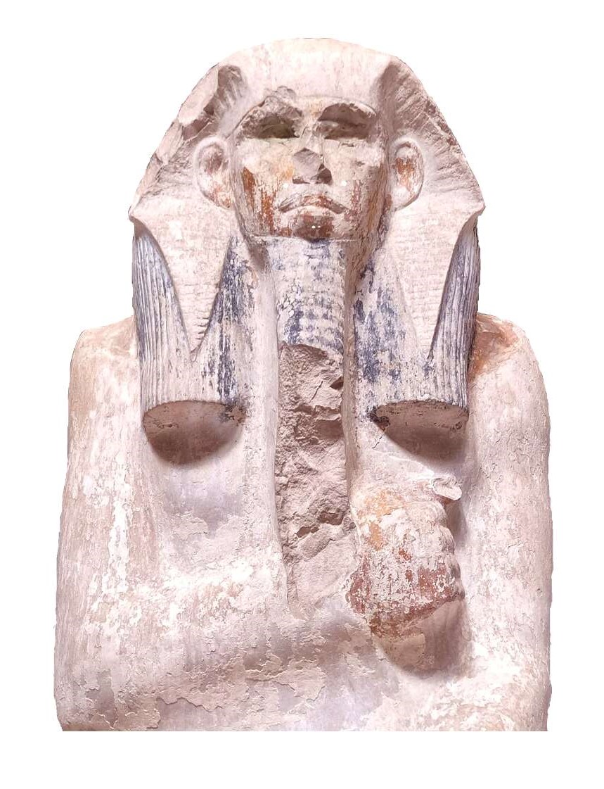
Djoser, who reigned during Egypt’s 3rd Dynasty (27th century BCE), forever transformed the landscape of ancient architecture. Guided by his brilliant vizier and architect Imhotep, Djoser commissioned the construction of the Step Pyramid of Saqqara, the first large-scale stone structure in human history. This bold innovation marked the beginning of Egypt’s pyramid age.

The Step Pyramid was more than a tomb, it was a statement of vision, ambition, and mastery over new techniques. Rising in six distinct tiers, it symbolized Egypt’s leap to the grand monuments that would define its civilization.
Inspired by the step by step analogy of Djoser’s Step Pyramid, Djoser Genomics is built on the foundation of transforming complex genomic data into clear, actionable insights, layer by layer, just like the pyramid itself.
📜 Codex Conclusion
With this scroll, we close the gates on our journey, a complete bulk RNAseq analysis pipeline told through the voices of ancient Egyptian figures.
From the silent sands of Saqqara with Djoser, Imhotep and Hesy-Ra, to the towering reigns of Khufu, Khafre, and Menkaure, and the Glories of Ramses II and Thutmose III, we have walked together inspired by those ancient figures to uncover the codex scrolls of bulk RNAseq.
You now hold the knowledge to process raw RNAseq data, align reads, quantify expression, find differentially expressed genes, and interpret them through biological pathways. Much like we approached GO and KEGG; GSEA adds another lens to see the story our genes are telling.
May these scrolls serve not just as instructions, but as companions in your own quests for discovery.
And as for what lies beyond these sands… 𓂀𓆣 well, some scrolls remain buried, waiting for the one who dares to uncover them 📜.
Papyrus Background from the Post’s Cover photo is from Freepik