Scroll 4: Khafre's Connections
Welcome to Scroll 4 of 8, from the Djoser’s Bulk RNAseq Tutorial Codex.
In this scroll, we bridge our quantified RNA-seq data to meaningful biological interpretation. Like King Khafre, who built enduring connections through his grand monuments and trade networks, we now establish crucial links between raw numbers and biological meaning.
With R as our foundation, we’ll set up our project, define our study design, bring in annotations from BioMart, and import Kallisto results with tximport, building the pathways that will guide our downstream analysis.
Note: This tutorial assumes you have basic experience with R, such as running commands, installing packages, and working with data frames. We will not be covering fundamental R syntax in detail.
📜 Scroll Objectives
- Prerequisites: Setting up R and RStudio
- Creating the Study Design
- Gene Annotations
- Fetching Annotations from Ensembl BioMart
- Importing Kallisto Results with Tximport
- Cultural Spotlight: Khafre – Builder of the Timeless Pyramid
Prerequisites: Setting up R and RStudio
For the downstream analysis in this scroll, we will be using R as our main analysis environment. Before proceeding, ensure you have:
- R installed on your system
- RStudio (optional but highly recommended) as your development environment
If you do not have R and RStudio installed yet, follow this video tutorial by DIY.Transcriptomics
Once both are installed, you’re ready to proceed. We’ll start by creating a new R Project and R script to keep our analysis organized.
Creating the Study Design
Before importing our quantification results into R, we need to define our study design. This serves as the blueprint for our analysis, to tell R which samples belong to which conditions and where their quantification files are stored.
We’ll use the tibble package to create a clean, readable table structure.
1
2
3
4
5
6
7
8
library(tibble)

# Creating Study Design file
studyDesign <- tibble(
  Accession = c("SRR24448340", "SRR24448339", "SRR24448338", "SRR24448337", "SRR24448336", "SRR24448335"),
  Sample = c("HS01", "HS02", "HS03", "CD01", "CD02", "CD03"),
  Condition = c("Healthy", "Healthy", "Healthy", "Disease", "Disease", "Disease")
)
- Accession: The Accession IDs for each sample.
- Sample: The short names we assigned during kallisto quantification.
- Condition: Biological condition for each sample (in this case, “Healthy” vs “Disease”).
We also need to make sure R handles our Condition column in studyDesign as a categorical variable.
1
2
# Ensuring Condition column in study design is categorical
studyDesign$Condition <- factor(studyDesign$Condition)
Then we can build paths for each dataset and ensure it is correct using the all(file.exists()) function
1
2
3
4
5
# Setting up Paths for kallisto abundance.tsv files
paths <- file.path('kallisto', studyDesign$Sample, 'abundance.tsv')

# Ensuring Paths are correct: Should return TRUE
all(file.exists(paths))
Gene Annotations
What are annotations?
In RNA-seq, quantification tools like kallisto produce counts for transcripts (e.g., ENST00000335137.4). While these transcript IDs are precise, they aren’t always intuitive, mostly we want to see gene names like BRCA1 for example.
Annotations bridge this gap by mapping transcript IDs to gene IDs and human-readable gene names.
Why do we need them?
- Convert technical transcript IDs into meaningful gene identifiers.
- Facilitate downstream analysis like differential expression at the gene level.
- Make visualizations and result tables understandable for researchers.
Fetching Annotations from Ensembl BioMart
We’ll use the biomaRt package to connect to the Ensembl database and retrieve annotation data.
1
2
3
4
5
6
7
8
9
10
library(biomaRt)
library(tidyverse)
library(dplyr)

# Setting up BioMart to get Annotations
myMart <- useMart(
  biomart = 'ENSEMBL_MART_ENSEMBL',
  dataset = 'hsapiens_gene_ensembl',
  host = 'https://www.ensembl.org'
)
useMart(...)Connects to the Ensembl BioMart database, specifying the human dataset.
1
2
# List available filters (optional, for exploration)
mart.filters <- listFilters(myMart)
listFilters(...)Lists possible filters you can apply when retrieving data (e.g., filter by chromosome or gene type).
1
2
3
4
5
6
7
8
9
10
11
12
13
14
15
# Accessing Human Annotations and selecting transcript id, gene id & gene name
annotations <- tryCatch({
  getBM(
    attributes = c('ensembl_transcript_id', 'ensembl_gene_id', 'external_gene_name'),
    mart = myMart
  ) %>%
    as_tibble() %>%
    dplyr::rename(
      target_id = ensembl_transcript_id,
      gene_id   = ensembl_gene_id,
      gene_name = external_gene_name
    )
}, error = function(e) {
  stop("Failed to fetch annotations from BioMart: ", e$message)
})
getBM(...)→ Fetches the actual annotation table containing:ensembl_transcript_id→ Transcript-level identifier (used by kallisto).ensembl_gene_id→ Gene-level identifier.external_gene_name→ Common gene name.
rename(...)→ Renames columns so that target_id matches kallisto’s output for easier merging later.
Importing Kallisto Results with Tximport
Now that we have annotations, the next step is to link our kallisto transcript counts to gene level counts.
We do this using the tximport package, which makes it easy to import quantification results into R for downstream analysis (e.g., DESeq2, edgeR).
Create the transcript to gene map
Kallisto outputs counts at the transcript level, but most downstream tools analyze gene level counts.
We therefore prepare a simple mapping table tx2gene (transcript 2 gene) with:
- target_id → Transcript ID (from kallisto output)
- gene_name → Human-readable gene symbol
1
2
3
# Creating tx2gene that contains only transcript id and gene name for tximport
tx2gene <- annotations %>%
  dplyr::select(target_id, gene_name)
Run tximport to aggregate counts
tximport reads the abundance.tsv files produced by kallisto and aggregates transcript counts into gene counts using our tx2gene mapping.
1
2
3
4
5
6
7
8
9
10
11
library(tximport)

# Running tximport
txi <- tximport(
  paths,                    # Paths to abundance.tsv files
  type = 'kallisto',         # Specify quantification tool
  tx2gene = tx2gene,         # Transcript-to-gene mapping
  txOut = FALSE,             # Summarize to gene level counts
  countsFromAbundance = 'lengthScaledTPM', # Adjust counts by transcript length
  ignoreTxVersion = TRUE     # Remove version suffix from transcript IDs
)
Explanation:
pathsList of file paths to kallisto’sabundance.tsvoutputs for each sample.type = 'kallisto'Tells tximport how to read the files.tx2geneMapping table we just created for converting transcript IDs to gene names.txOut = FALSEOutput gene-level counts rather than transcript-level counts.countsFromAbundance = 'lengthScaledTPM'Recommended normalization that adjusts counts by transcript length and abundance.ignoreTxVersion = TRUEStrips version numbers from Ensembl transcript IDs for matching.
Outcome:
You now have a gene-level expression matrix stored in txi, ready for differential expression analysis and visualization.
If you want to continue, head over to the next scroll: Menkaure’s Measures, where we’ll perform differential expression analysis (DEA) using DEseq2.
Time for our Cultural Spotlight!
🏛️ Cultural Spotlight: Khafre – Builder of the Timeless Pyramid
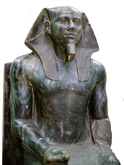
Khafre, also known as Chephren, was a ruler of Egypt’s Fourth Dynasty. He was the son of Khufu, the builder of the Great Pyramid, and carried forward his family’s ambitious tradition of monumental construction.

His pyramid at Giza, though slightly smaller in base than his father’s, was built on higher ground, creating the illusion that it matched or even exceeded Khufu’s in height. Uniquely, the topmost layers of its original Tura limestone casing are still visible today, offering a rare glimpse of how these structures once gleamed in the desert sun.

Khafre’s complex also includes the Great Sphinx of Giza, widely believed to bear his likeness, guarding the pyramid for eternity.
Papyrus Background from the Post’s Cover photo is from Freepik