Scroll 3: Khufu's Calculations
Welcome to Scroll 3 of 8, from the Djoser’s Bulk RNAseq Tutorial Codex.
In this scroll, we perform pseudoalignment, a fast, reference-based mapping approach, to quantify transcripts from our RNA-seq reads. Like Khufu, the visionary behind the Great Pyramid, we rely on efficient design and foundational precision to build something monumental.
Let’s begin the alignment.
📜 Scroll Objectives
- What Is Alignment, and Why Do We Do It
- Common Tools for Alignment
- What is Pseudoalignment, and How Does It Differ from Alignment
- When is Pseudoalignment the Better Option?
- Installing Kallisto on Google Colab
- Reference Transcriptome Indexing using Kallisto
- Quantifying Expression with Kallisto
- Alignment Rate Check (Quality Control)
- Cultural Spotlight: Khufu – Mastermind of the Great Pyramid
What Is Alignment, and Why Do We Do It?
Before we push forward in our transcriptomics journey, we must first pause, and understand the concept of sequence alignment.
In RNA-seq analysis, after sequencing, we’re left with millions of short reads. But they’re just disconnected fragments. To make sense of them, we need to reconnect them to their original source: a reference genome or in our case a reference transcriptome.
That’s what alignment does: It takes each read and finds the best-matching location in the genome or transcriptome, to help us understand where does this fragment come from in our genome or transcriptome
Common Tools for Alignment
These tools use algorithms to search for where reads fit:
- HISAT2 – Fast, memory-efficient, often used for genome alignment.
- STAR – Extremely fast and splice-aware, ideal for eukaryotic transcriptome data.
- BWA – Great for DNA reads, used often in genomics pipelines.
But there’s a catch, Alignment is powerful, but also computationally expensive. It can take hours, require a strong CPU, computational power and produce huge files (like BAMs). For large datasets or limited compute resources, it becomes a bottleneck.
That’s where King Khufu would raise an eyebrow, and perhaps suggest a more efficient architectural strategy.
What is Pseudoalignment, and How Does It Differ from Alignment?
Pseudoalignment skips the base-by-base matching. Instead, it identifies which transcripts a read could have originated from, without determining its exact position. It uses k-mers (short subsequences of length k) from the reads and compares them to a k-mer index of the transcriptome.
Think of it like asking: “Does this read belong to transcript X, Y, or Z?” rather than: “Where exactly does this read align in the genome?”
The two most widely known pseudoaligners are:
- Kallisto – The tool we’ll be using in this scroll.
- Salmon – Another fast and flexible pseudoaligner.
When is Pseudoalignment the Better Option?
Pseudoalignment is a great choice when:
- Your goal is quantification, estimating transcript/gene expression levels, not variant calling or splicing analysis.
- You want speed and efficiency, it can process large datasets much faster than traditional aligners.
- You have limited computational resources, pseudoalignment uses less RAM and CPU.
However, it’s not suitable if you need:
- Precise read locations on the genome.
- Working on splicing.
- Using any other tools that use BAM alignment files.
For bulk RNA-seq focused on quantification, pseudoalignment offers an optimal balance between speed and accuracy, which is exactly why we’re using Kallisto in this tutorial.
If you want to learn more about alignment vs pseudoalignment (Kallisto), check out this Awesome Video from DIY.transcriptomics.
Installing Kallisto on Google Colab
To run Kallisto in Google Colab, we need to install it manually using Conda.
Step 1: Install Conda (Miniconda)
We’ll begin by downloading and installing Miniconda, a lightweight version of Conda:
1
2
3
4
# Install Miniconda
!wget https://repo.anaconda.com/miniconda/Miniconda3-latest-Linux-x86_64.sh
!chmod +x Miniconda3-latest-Linux-x86_64.sh
!./Miniconda3-latest-Linux-x86_64.sh -b -f -p /usr/local
This code does the following:
wgetdownloads the Miniconda installer.chmod +xgives execute permissions.- The
./command installs it to/usr/local
Then verify the installation:
1
2
# Verify Conda installation
!conda --version
Step 2: Update Environment Variables
After installing Miniconda, we need to ensure that the Conda commands are recognized in our Colab environment.
1
2
import os
os.environ['PATH'] = '/usr/local/bin:' + os.environ['PATH']
This code makes sure Conda commands are recognized and can be used inside the Colab environment.
Step 3: Add Conda Channels
We’ll add the required Conda channels to access bioinformatics tools:
1
2
3
!conda config --add channels defaults
!conda config --add channels bioconda
!conda config --set offline false
defaultsis the main Conda channel.biocondacontains bioinformatics software like Kallisto.
We also make sure Conda won’t default to offline mode.
You can confirm the channels were added:
1
!conda config --show channels
Step 4: Install Kallisto
Now install Kallisto directly from Bioconda:
1
!conda install -c bioconda kallisto -y
The -y flag auto confirms installation prompts.
Finally, test that it is successfully installed:
1
!kallisto
Reference Transcriptome Indexing using Kallisto
Before we can pseudoalign RNA-seq reads using Kallisto, we need to create an index from a reference transcriptome. The index enables Kallisto to rapidly locate the origin of reads.
What is Indexing?
Indexing is the process of converting a FASTA reference file into a structured, searchable format that the aligner or pseudoaligner can use for quick read assignment.
For Kallisto, the input reference is usually a cDNA (transcript level) FASTA file, not the full genome. This is because Kallisto performs transcript level quantification.
Without indexing, Kallisto would have to scan the entire reference file for every read, this would be very slow and computationally inefficient. The index accelerates the process by using k-mer hashing.
Creating the Reference Transcriptome Index
First we will Unzip the FASTA file if it’s compressed (.gz).
1
2
# Unzipping the reference FASTA
!gunzip "/content/RNAseq/Homo_sapiens.GRCh38.cdna.all.fa.gz"
Then we will use !kallisto index to create the index file.
1
2
3
4
5
6
7
8
9
# Defining file paths
fasta_file = os.path.join(folderPath, "Homo_sapiens.GRCh38.cdna.all.fa")
index_file = os.path.join(folderPath, "Homo_sapiens.GRCh38.cdna.all.index")

# Creating the kallisto index
!kallisto index -i {index_file} {fasta_file}

# Confirming success
print(f"Index created: {index_file}")
Quantifying Expression with Kallisto
Once the reference transcriptome index is prepared, it’s time to quantify transcript abundances for each sample using Kallisto’s quant command.
kallisto quant takes your indexed reference and your raw FASTQ files and performs psuedoalignment to estimate how many transcripts are present in each sample, quickly and efficiently.
Sample Setup
We define a list of our samples with corresponding FASTQ files:
1
2
3
4
5
6
kallistoData = [['HS01', 'SRR24448340.fastq.gz'],
                ['HS02', 'SRR24448339.fastq.gz'],
                ['HS03', 'SRR24448338.fastq.gz'],
                ['CD01', 'SRR24448337.fastq.gz'],
                ['CD02', 'SRR24448336.fastq.gz'],
                ['CD03', 'SRR24448335.fastq.gz']]
- HS samples are healthy controls.
- CD samples are from cardiac disease patients.
The HS and CD prefixes help us differentiate between healthy and disease samples, which is crucial for downstream analysis, You can know which sample is which through the sample metadata of each one on ENA.
Run Kallisto for Each Sample
Let’s Create our main Output folder for Kallisto results:
1
mkdir RNAseq/kallisto
Then we run quantification with the following code:
1
2
3
4
5
6
7
8
9
for data in kallistoData:
  folder = os.path.join(folderPath, f"kallisto/{data[0]}")
  filelocation = os.path.join(folderPath, data[1])

  !kallisto quant \
  -i {index_file} \
  -o "$folder" \
  --single -l 250 -s 30 \
  "$filelocation"
Explanation:
-i {index_file}: The path to the reference transcriptome index you created earlier.-o "$folder": Output folder for results (TPMs and estimated counts).--single: Specifies that the reads are single-end.-l 250 -s 30: Estimated average fragment length and standard deviation (important for single-end data)."$filelocation": Input FASTQ file.
Outcome:
Each sample will now produce a folder containing kallisto quant output including a file named abundance.tsv, which includes:
- Estimated counts
- TPMs (Transcripts Per Million)
- Effective lengths
Alignment Rate Check (Quality Control)
Before moving forward, it’s essential to check the alignment rate for each sample. It can be found in the run_info.json file inside each sample’s output directory.
Open the run_info.json file and look for the p_pseudoaligned field. A good alignment rate is typically above 70–80%. Low alignment percentages might indicate issues like:
- Poor-quality reads
- Contamination
- Incorrect transcriptome index
⚠️ If alignment rates are unusually low, consider rechecking your FASTQ files or the transcriptome reference.
That’s it! You can now download the kallisto folder from the left sidebar in Google Colab.
You now have quantification results for all samples, ready to be imported into R for downstream analysis and visualization!
If you want to continue, head over to the next scroll: Khafre’s Connections, where we’ll import our data into R, Fetch our annotations and Create our study Design.
Now time for our next Cultural Spotlight.
🏛️ Cultural Spotlight: Khufu – Mastermind of the Great Pyramid
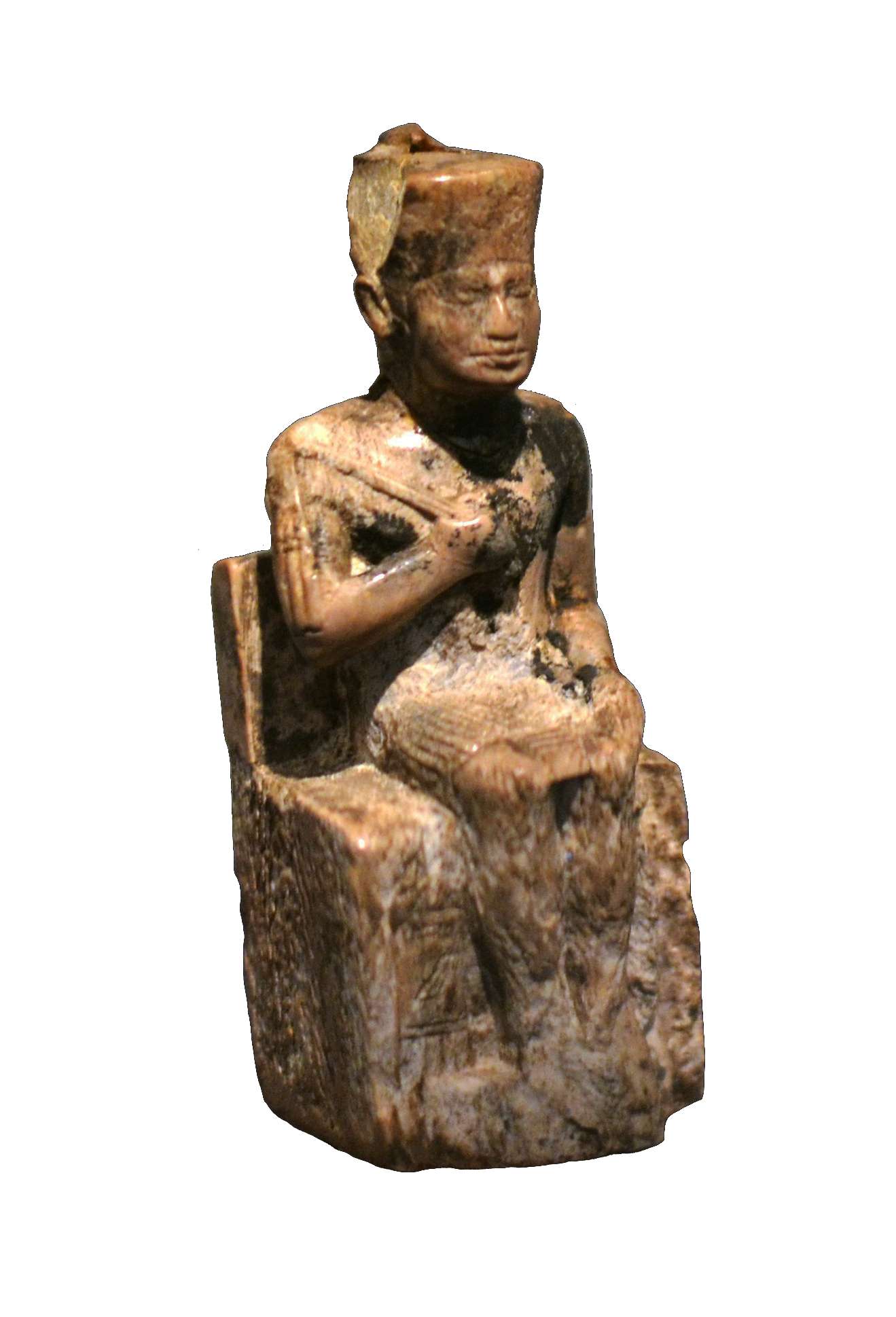
As we align sequences with surgical precision, let’s spotlight a figure known for monumental precision, King Khufu (c. 2600 BC). Also known as Cheops, Khufu was the pharaoh behind the construction of the Great Pyramid of Giza, the largest and most iconic pyramid in Egypt.

Khufu’s pyramid stood as the tallest human-made structure on Earth for over 3,800 years, a true feat of ancient engineering, planning, and coordination. Much like genome indexing prepares the way for efficient data alignment, Khufu’s pyramid was a meticulously planned foundation that shaped architectural history.
Papyrus Background from the Post’s Cover photo is from Freepik